What is Considered to be Random?

2020-08-16

We all have heard of prominent artists such as Jackson Pollock that at first sight on their work did not appreciate the complexity and level of intricacy in their pieces. One, without taste of art (and math!) might foolishly claim that they can reproduce similar patterns since there are actually none! It looks random. but what does “random” actually mean?¹ A word that has been thrown around carelessly in daily life which contain variety of meanings. If you think about it really, it’s not so obvious how to actually define “random” rigorously and it’s been a matter of debate for a long time in probability theory.

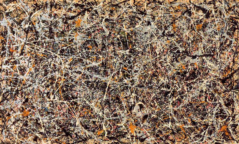
Autumn Rhythm by J. Pollock

Historically, probability has it’s roots in gambling and safe to say that its classical form was developed by gamblers to enhance their gaming strategies! In addition, probability theory in its early stages was built upon counting and combinatorics. Probability associated to events were simply defined as number of desirable cases over total number of cases which would result in a rational fraction. People would have laughed at you if you’ve said that you have a biased coin with $p = \frac{1}{\sqrt{2}}$ or any other irrational number. Surprisingly, a physician named G. Cardano was first to conjecture that some sort of Law of Large Numbers should rule random sequences (of independent trials) to provide a practical meaning, and was later proved rigorously by Bernoulli.² In fact, this law opened a window in which you can associate even irrational probabilities to events since any irrational number can be well approximated by rational fractions. All this has led to a frequency point of view of probability which was the bridge between mathematics and real world, and later allowed statisticians to do inference.

What Does Probability of an Event Mean in Practice?

A circular approach

What do we mean by having a fair coin? Well, one explanation is that the outcome of the tossed coin is unpredictable to us and we have no preference over each side. This statement, although true, is nevertheless subjective and one might even say they do have the capability to predict the outcome. How can we fact check that? Naturally, one would replicate the experiment multiple times and somehow compare the predicted and real outcomes. This is the point where things get a little circular. In order to give universal meaning to probability you need multiple outcomes of that coin tossing experiment with the same randomness; In other words, generated independently and identically. Randomness is only practically meaningful through replication and that was the main motivation to define it theoretically in such a way to conform to this idea.³

This sort of argument is analogous to say 1 object is only meaningful if there exists 2 of them besides together, moreover 1+1=2. Thus, 1 is tied to the whole integer system and they are not meaningful individually.

A Rigorous Attempt to Define Randomness

Suppose $\Omega=\{0,1\}^\mathbb{N}$ be the outcome space associated to the sequence of a coin tossed infinitely many times, denoted as $X_1,X_2, \dots$. Indeed, we assume trials are performed independently, i.e. $(X_n)_{n\ge1}$ are independent random variables.⁴ It is common to consider independence provides chaos in the sequence and makes it irregular since there are no sensible dependency among the variables, however it’s the very thing that adds some sort of limiting structure to the sequence. This structure ensures that a random sequence must satisfy some sort of frequency stability condition, and suggests to define randomness upon this crucial condition. The necessity of this condition is evident, however the more appropriate question is “Is this property sufficient?”.

Definition. A binary sequence $X=(X_n)_{n \ge 1}$ is considered to be random if it has the following properties:

(Frequency Stability) let $f_n = X_1 + \dots+X_n$ be the number of 1s among first $n$ terms. Then: \[ \lim_{n \mapsto \infty}{\frac{f_n}{n}} = p \] exists and $0<p<1$.
Suppose $\Phi$ is a rule for selecting a subsequence of $X$ such that $X_n$ is chosen iff $\Phi(X_1,\dots,X_{n-1})=1$. Then the subsequence obtained via this rule must satisfy the aforementioned property with the same $p$.

As discussed previously, the first property is known as the Law of Large Numbers. The second property, although looks mysterious, simply states that valid subsequences should also satisfy frequency stability since after all they are a sub-collection of i.i.d. random variables. It also has an interpretation in gambling called Laws of Excluded Gambling Strategy Strategy. Indeed, every subsequence won’t work; For instance, if you look at the subsequence that they are all 0s or all 1s then stability will not hold. In the rest of this article we will adopt this notion of randomness as our definition.

Perception of Randomness

In this section we are mainly interested in understanding how human intuition perceives randomness. What type of features in a sequence would trigger human’s intuition as chaotic? Suppose I give you a binary sequence and ask you to judge about whether this sequence was generated uniformly random or not. Can you find meaningful patterns in it? Which one of the following sequences appears to be random in your perspective?

\[\{H,T,H,H,T,H,T,H,H,H,T,H,T,H,H,T,H,H,T,T,H,T,H,H,T\}\] \[\{H,T,H,H,H,H,T,H,T,T,H,T,H,H,H,H,H,T,H,T,T,T,T,T,T\}\] These type of questions are rather difficult to answer in a polarized manner. However, there are quantitative methods to answer them in a spectrum. In statistics, we usually call it Hypothesis Testing which itself has a long history. Psychologists found that people’s notion of randomness is rather biased in the sense that they see streaks in a truly random sequence and expect more alternation, or shorter runs, than are there. They tend to pay more attention toward frequency stability rather than other patterns. Examples of such misleading fallacies in gambling can be found in “53 Fever” which led 4 billion euros worth of bet to be wasted. This phenomena makes sense in a way that the actual mathematical definition relies heavily on frequency stability but the issue is you are provided with only a partial sequence and not an infinite one. This is the part that you have to be more clever and extract some extra features to make your final judgment.

Streaks of What Length Should we Expect In a Random Sequence of Length n?

Let us define stopping time $T_{k}$ to be the first time that we observe a streak of ones with length $k$ in our infinite sequence. Therefore, one should expect existence of streaks with length $k$ in a sequence of length $\mathbb{E}[T_{k}]$. For the sake of clarity, let us also define $\mathcal{F}_{T_k}$ to be filtration up to stopping time $T_{k}$, i.e. $\mathcal{F}_{T_k} = \sigma(X_1,\dots,X_{T_k})$. Then, we have the following: \[ \mathbb{E}[T_k|\mathcal{F}_{T_{k-1}}] = \frac{1}{2}(1+T_{k-1}) + \frac{1}{2}(1+T_{k-1} + \mathbb{E}[T_k])\] This is due to the fact that a streak of length $k-1$ must occur before than a streak of length $k$. Therefore, at time $T_{k-1}+1$ either we are done by observing a 1 or everything resets to a new sequence by observing a 0.⁵ Now by taking expectations from both sides we obtain this recursive equation:

\[ \mathbb{E}[T_k] = 2(1+\mathbb{E}[T_{k-1}])\] With initial condition $T_{0} = 0 $ which has this solution:

\[ \mathbb{E}[T_k] = 2^{k+1}-2 \]

At this point, an interesting question would be whether this random variable is concentrated around it’s mean or not? if so, how well? Apparently this does not seem to be true and $T_{k}$ tends to have a heavy tailed distribution.

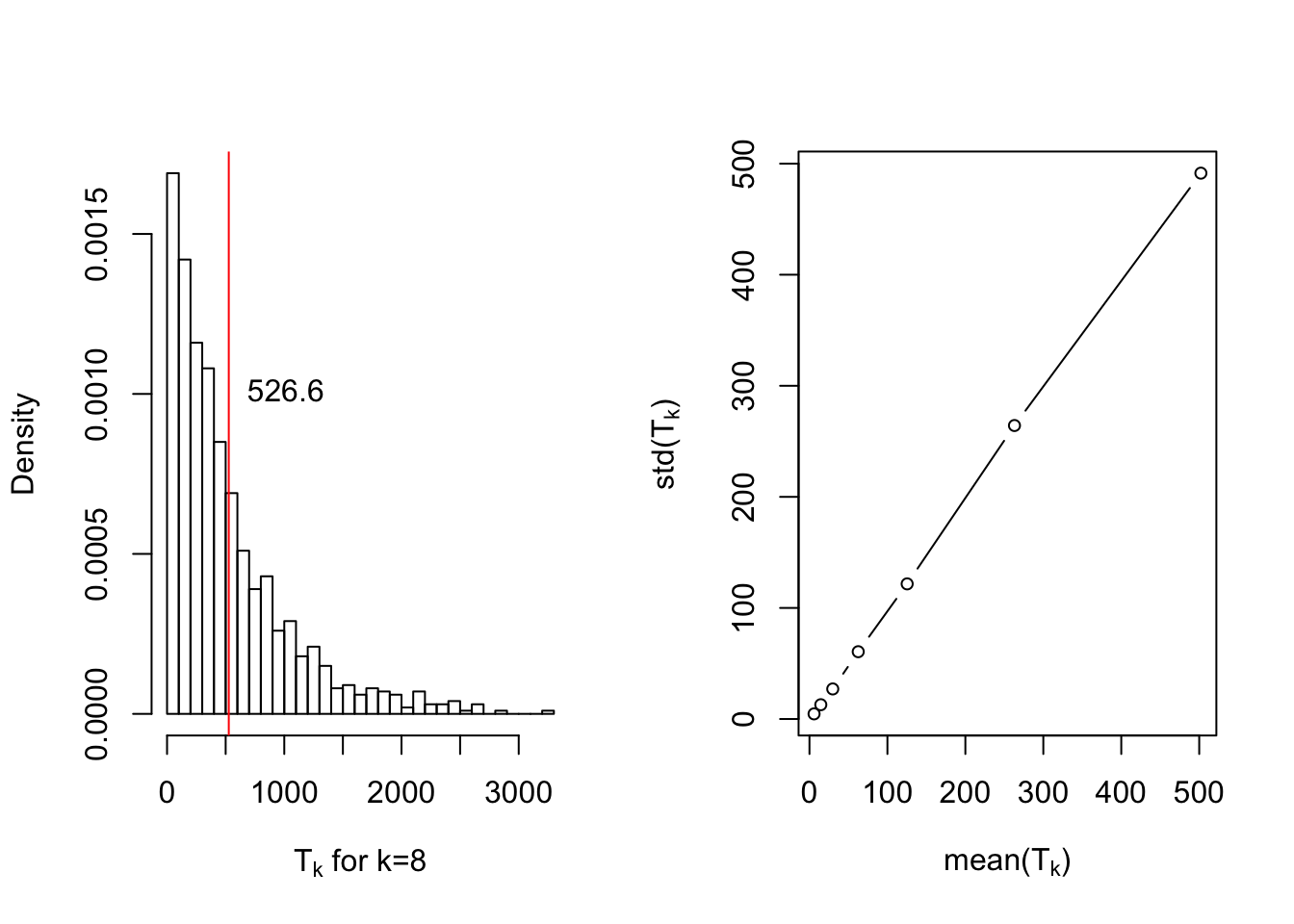
In conclusion, one should expect a streak of length $\log_2(n)$ in a fair random sequence. Thus, for those of you who was suspicious toward the second provided sequence due to long runs, I must say you were wrong.

Wald and Wolfowitz Test

Myriad number of tests were developed to quantify randomness in a sequence. After all, this is an important problem since fields such as cryptography relies heavily on the randomness assumption which guarantees existence of codes that are intractable to break. Some tests are based on the longest run in the sequence, while others as in Wald and Wolfowitz test are based on the number of runs.

Instead of binary, let us assume $\Omega = \{+1,-1\}^\infty$ which allows us to easily detect changes in the sequence. Thus, we can define $R_n$ to be the number of runs in a sequence of length $n$ and can be expressed explicitly in the following way:

\[ R_{n} = 1 + \sum_{t=2}^{n}{\frac{1-X_{t}X_{t-1}}{2}} \] Note that $R_{n}$ consist of sums of $n-1$ independent random variables, and therefore CLT can be applied. Subsequently, one can design a test to reject the null hypothesis $H_0$ when the following statistics is too large in absolute value and obtain a p-value. \[ \frac{R_n - \mathbb{E}[R_n]}{Var(R_n)} = \frac{1}{\sqrt{n-1}}\sum_{t=2}^{n}{X_{t}X_{t-1}} \overset{n \mapsto \infty}{\longrightarrow} \mathcal{N}(0,1) \]

Now, if we apply this test to the given sequences we observe that the latter looks to be significantly more random than the former which is counter-intuitive.

	First.Sequnce	Second.Sequnce
P Value	0.0412268	0.6830914

This does not necessarily mean, our test was wrong or we got bad luck, but could simply mean that our intuition is not fully aligned with the intended notion of randomness. As much as human perception of randomness could be biased, generating something that looks random is difficult. It is also worth mentioning that this entire discussion was 1-dimensional and mainly focused on 1-dimensional local features such as streaks. However, one should expect novel and astonishing phenomena to occur even in 2-dimensions since human intuition is now equipped with 2-dimensional local neighborhood.

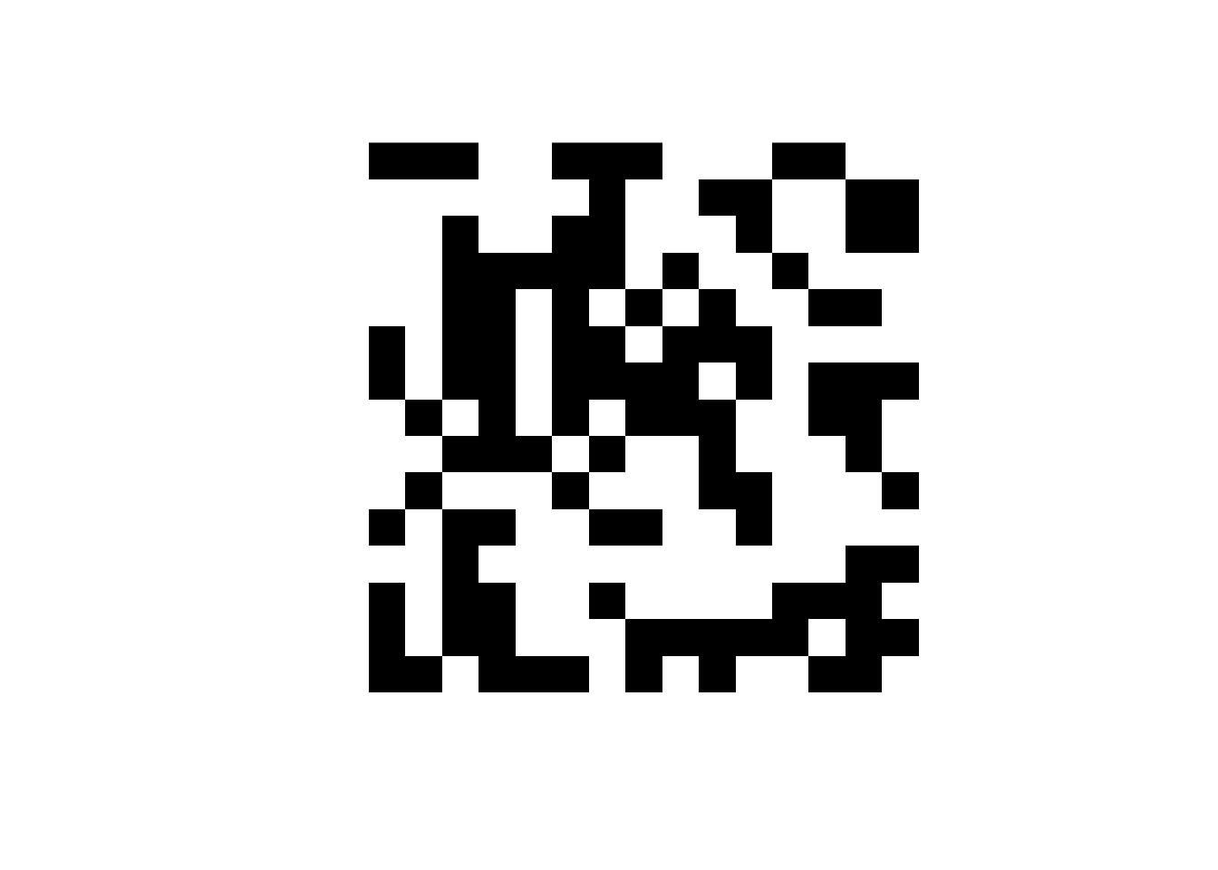Phenomena such as percolation which states that there is a path from center to the border of a random 2-dimensional matrix with black and white pixels is of particular interest to me and I’ll write about them in the near future.

A rigorous explanation can be found here ↩
Some Laws and Problems of Classical Probability and How Cardano Anticipated Them ↩
It is fair to say independence itself is not well defined in practice. Do we mean to conduct our experiment with exact same conditions? Shouldn’t that make the outcome identical to the previous experiment? This is indeed a matter of debate in philosophy of probability, and frankly, don’t know the answer to it.↩
A pedantic reader might also be skeptical about this statement since it’s not trivial to define independence over an infinite collection of random variables and it’s true. It requires further knowledge in measure theory but for now consider it means every finite sub-collection should be independent↩
This reset argument is rather technical and it’s due to the Strong Markov Property of discrete Markov Chains which states that $(X_{T+n})_{n \ge 1}$ is again a Markov Chain with the same transition probability provided that $T$ is a stopping time.↩