Sharp Bounds on Spectral Norm of a Random Matrix

2020-08-22

notes

Random Matrix Theory Probability , Measure Concentration

Singular values of matrices show up in many different places, and studying them has significant importance in math. As per usual, it has a fairly simple definition but requires quite diffficult tools to analyze comprehensively. In this article I aim to demonstrate how would norm of a Gaussian random matrix behave and answer questions such as “How does it’s mean behave?” or “Is it concentrated around it’s mean?”. A crucial assumption employed on the entries of $A$ is independence. Indeed, the results can be extended easily to subgaussians as well, however stating theorems with gaussians evaporates the annoying constants! Let’s set up some notations, shall we?

Definition. For any matrix $A \in R^{n \times m}$ we define spectral norm (i.e. largest singular value) as: $| | A | |_{o p} = max_{\begin{matrix} u \in S^{n - 1} \\ v \in S^{m - 1} \end{matrix}} ⟨ u, A v ⟩$

It is worth mentioning, the reason that I exchanged maximum instead of suprema is merely because suprema of a continuous function will be achieved on a compact set. This norm is a measure of how much a vector can be dialated through the linear transform $x \mapsto A x$ in the worst case.

Definition. An unbiased random variable $X$ is called $σ^{2}$ -subgaussian if one of the following holds.¹ Moreover, all the statements are equivalent with different constants:

(Moment Generating Bound) $E [e^{t X}] \leq e^{\frac{t^{2} σ^{2}}{2}}$ for all $t \in R$ .
(Tail Bound) $P [| X | \geq t] \leq 2 e^{- \frac{t^{2}}{2 σ^{2}}}$ for all $t \geq 0$ .
(Moment Bound) $| | X | |_{L^{p}} = (E [X^{p}])^{\frac{1}{p}} \leq σ \sqrt{p}$ for all $p \geq 1$ .
(Another MGF Bound) $E [e^{\frac{X^{2}}{2 σ^{2}}}] \leq 2$

In a nutshell, this property is roughly saying that the random variable behaves like a normal and it is desirable since it’s basically equivalent to concentration around mean (or median). For fixed vectors $u \in S^{n - 1}, v \in S^{m - 1}$ one can easily check that $X_{u, v} = ⟨ u, A v ⟩$ is also sub-gaussian with the same parameter of entries of $A$ , thus concentrated around it’s mean. However, it’s not clear what can be said about suprema of this collection of random variables which is the quantity of interest.² Note that these random variables are locally correlated, i.e. for a pair $(u^{^{'}}, v^{^{'}})$ close to $(u, v)$ we expect $X_{u, v}$ to be close to $X_{u^{^{'}}, v^{^{'}}}$ . More precisely, one can write: $| X_{u, v} - X_{u^{^{'}}, v^{^{'}}} | \leq | X_{u, v} - X_{u^{^{'}}, v} | + | X_{u^{^{'}}, v} - X_{u^{^{'}}, v^{^{'}}} | \leq | | A | |_{o p} (| | u - u^{^{'}} | | + | | v - v^{^{'}} | |)$ Surprisingly, the inverse is also true meaning if one take two pairs far apart from each other the corrseponding random variables will also be uncorrelated, thus behave as though they were independent since uncorrelatedness is equivalent to independence in gaussian fields. This sort of argument motivated proofs based on $ϵ$ -net methods which I do not intend to go through here, however the intuition is very insightful. In order to make this statement more precise one may use the following comparison inequality for gaussian random variables.

Theorem (Sudakov-Fernique Inequality). Suppose $X, Y \in R^{n}$ are two independent centered Gaussian vectors such that $E [| X_{i} - X_{j} |^{2}] \leq E [| Y_{i} - Y_{j} |^{2}]$ for $\forall i, j \in [n]$ . Then: $E [max_{i \leq n} X_{i}] \leq E [max_{i \leq n} Y_{i}]$ As a special case if we assume that $X, Y$ has the same variance coordinatewise, then the condition in the theorem verbally translates into $X$ is more correlated than $Y$ , thus should possess a lower maximum which aligns with intuition.³ In addition, it is easy to extend this to infinite case using a simple truncation and then applying monotone convergence theorem provided that the index set is seperable. I am not going to provide a proof for this theorem here since the ideas overlap with the theorems mentioned below but this theorem has an direct application to upper bounding spectral norm of a matrix. Take $X_{u, v}$ as defined above and assume entries of matrix $A$ has standard normal distribution: $\begin{aligned} E [| X_{u, v} - X_{u^{^{'}}, v^{^{'}}} |^{2}] & = E [| \sum_{\begin{array}{c} i \in [n] \\ j \in [m] \end{array}} (u_{i} v_{j} - u_{i}^{^{'}} v_{j}^{^{'}}) A_{i, j} |^{2}] = \sum_{\begin{array}{c} i \in [n] \\ j \in [m] \end{array}} (u_{i} v_{j} - u_{i}^{^{'}} v_{j}^{^{'}})^{2} \\ = \sum_{\begin{array}{c} i \in [n] \\ j \in [m] \end{array}} (u_{i} v_{j} - u_{i}^{^{'}} v_{j})^{2} + (u_{i}^{^{'}} v_{j} - u_{i}^{^{'}} v_{j}^{^{'}})^{2} + 2 u_{i}^{^{'}} v_{j} (u_{i} - u_{i}^{^{'}}) (v_{j} - v_{j}^{^{'}}) \\ = \sum_{i \in [n]} (u_{i} - u_{i}^{^{'}})^{2} + \sum_{j \in [m]} (v_{j} - v_{j}^{^{'}})^{2} + 2 \underset{\leq 0}{\underset{⏟}{\sum_{i \in [n]} u_{i}^{^{'}} (u_{i} - u_{i}^{^{'}})}} \underset{\geq 0}{\underset{⏟}{\sum_{j \in [m]} v_{j} (v_{j} - v_{j}^{^{'}})}} \\ \leq \sum_{i \in [n]} (u_{i} - u_{i}^{^{'}})^{2} + \sum_{j \in [m]} (v_{j} - v_{j}^{^{'}})^{2} \end{aligned}$ Now, one can define the following process for independent random variables $G \sim N (0, I_{n \times n})$ and $G^{^{'}} \sim N (0, I_{m \times m})$ as: $Y_{u, v} = ⟨ u, G ⟩ + ⟨ v, G^{^{'}} ⟩ \forall u \in S^{n - 1}, v \in S^{m - 1}$ Therefore, by Fernique’s inequality we obtain: $E [| | A | |_{o p}] = E [sup_{\begin{matrix} u \in S^{n - 1} \\ v \in S^{m - 1} \end{matrix}} X_{u, v}] \leq E [sup_{\begin{matrix} u \in S^{n - 1} \\ v \in S^{m - 1} \end{matrix}} Y_{u, v}] = E [| | G | |] + E [| | G^{^{'}} | |] \leq \sqrt{m} + \sqrt{n}$ This is a sharp upper bound when $m = Ω (n)$ since we can lower bound spectral norm by the norm of its first column: $E [| | A | |_{o p}] \geq E [sup_{u \in S^{n - 1}} X_{u, e_{1}}] = E [| | A_{:, 1} | |] ≳ \sqrt{n}$ Now that we established a sharp behaviour of largest singular value in expectation we move onto the next question on the list which is how well this quantity is conentrated around its mean?

A Hammer (Lipschitz Concentration)

Before we continue, we need to introduce a powerful tool which is widely used in the literature of measure concentration. Suppose $γ_{n}$ is $n$ -dimensional Gaussian measure where expectation is deonted by $γ_{n} f = E_{γ_{n}} [f]$ for $f : R^{n} \mapsto R$ . Then Poincaré’s inequality suggest that functions with small local variations should expect small variances. In other words, some sort of gradient of the function as an indication of local fluctuation can be translated into a bound on global fluctuation. $V a r (f) \leq E [| | \nabla f | |_{2}^{2}]$ This mainly suggest that one should expect dimension-independent concentration bounds for Lipschitz functions.

Theorem. Suppose $f : R^{n} \mapsto R$ is a $κ$ -Lipschitz function. Then, we have the following concentration inequality: $γ_{n} {| f - γ_{n} f | \geq t} \leq 2 e^{- \frac{t^{2}}{2 κ^{2}}}$ There are in fact many ways to approach this problem namely Interpolation Method due to Pisier-Mauray, Smart Path due to Talagrand, Isoperimetry due to Borell and Sudakov, Transporation Method due to Marton, etc.⁴ However, I will provide a neat proof usng Stochastic Calculus which is mathematically beautiful but may seem like a magical juggling performed by the very Brownian Motion! Honestly, I get super excited whenever Brownian Motion comes up and it almost never disappoints.

Proof. (Requires Knowledge in SDE)

Proof. The idea is to think of our gaussian vector as a point from a $n$ -dimensional brownian path $B_{t}$ at time 1 and define the martingale $M_{t} = E [f (B_{1}) | F_{t}]$ which interpolates continuously between $M_{0} = γ_{n} f$ and $M_{1} = f (B_{1})$ . Since, Brownian Motion is also a Markov Process we can rewrite $M_{t}$ as $E [f (B_{1}) | B_{t}] = F (t, B_{t})$ where $F$ is a smooth function and in fact inherits smoothness properties of $f$ .⁵ Assuming it’s valid to exchange integration and differentiation, one can write: $\begin{aligned} | | \nabla_{B_{t}} F (t, B_{t}) | | & = | | \nabla_{B_{t}} E [f (B_{1} - B_{t} + B_{t}) | B_{t}] | | \\ = | | E_{G} [\nabla_{B_{t}} f (\sqrt{1 - t} G + B_{t})] | | \\ \leq E_{G} [| | \nabla_{B_{t}} f (\sqrt{1 - t} G + B_{t}) | |] \leq κ \end{aligned}$ where the last inequality is due to Jensen’s inequality. Thus, we can now use Fundamental Theorem of Calculus and write the difference $M_{1} - M_{0}$ as an integral of $d M_{t}$ and this is the part Ito’s Formula kicks in: $d M_{t} = \frac{\partial}{\partial t} F (t, B_{t}) d t + \sum_{i = 1}^{n} \frac{\partial}{\partial B_{t, i}} F (t, B_{t}) d B_{t, i} + \frac{1}{2} \sum_{i, j} \frac{\partial^{2}}{\partial B_{t, i} \partial B_{t, j}} F (t, B_{t}) d ⟨ B_{, i}, B_{, j} ⟩_{t}$ Where $⟨ X, Y ⟩$ is the quadratic variation of two $L^{2}$ martingales such that $X Y - ⟨ X, Y ⟩$ is again martingale. Now quadratic variation between coordinate $i$ and $j$ is zero due to independence for distnct $i, j$ . However, by the uniqueness of quadratic variation for $i = j$ we have: $E [B_{t, i}^{2} - t | F_{s}] = E [(B_{t, i} - B_{s, i} + B_{s, i})^{2} - t | F_{s}] = B_{s, i}^{2} - s$ Thus, $⟨ B_{, i}, B_{, i} ⟩_{t} = t$ and we obtain: $d M_{t} = \sum_{i = 1}^{n} \frac{\partial}{\partial B_{t, i}} F (t, B_{t}) d B_{t, i} + (\frac{\partial}{\partial t} F (t, B_{t}) + \frac{1}{2} \sum_{i} \frac{\partial^{2}}{\partial B_{t, i}^{2}} F (t, B_{t})) d t$ Since $M$ is martingale the second term (which has finite variation) must be zero which implies that $F$ satisfies heat equation and again we can rewrite: $M_{t} - M_{0} = \sum_{i = 1}^{n} \int_{0}^{t} \frac{\partial}{\partial B_{t, i}} F (t, B_{t}) d B_{t, i}$

Now by linearity of quadratic variations: $\begin{aligned} ⟨ M ⟩_{t} & = \sum_{i, j} \int_{0}^{t} \frac{\partial}{\partial B_{t, i}} F (t, B_{t}) \frac{\partial}{\partial B_{t, j}} F (t, B_{t}) d ⟨ B_{, i}, B_{, j} ⟩_{t} \\ = \sum_{i = 1}^{n} \int_{0}^{t} | \frac{\partial}{\partial B_{t, i}} F (t, B_{t}) |^{2} d t = \int_{0}^{t} | | \nabla F (t, .) | |^{2} d t \leq κ^{2} t \end{aligned}$

This might not seem significant however a lot of information is burried deep within it. Again using Ito’s formula one can prove that the following process is a martingale:

Z_{t} = e^{λ M_{t} - \frac{λ^{2}}{2} ⟨ M ⟩_{t}} \geq e^{λ M_{t} - \frac{λ^{2} κ^{2}}{2} t}

Therefore:

e^{λ γ_{n} f} = e^{λ M_{0}} = E [Z_{0}] = E [Z_{1}] \geq E [e^{λ f (B_{1}) - \frac{λ^{2} κ^{2}}{2}}]

Now by rearranging terms:

E [e^{λ (f - γ_{n} f)}] \leq e^{\frac{λ^{2} κ^{2}}{2}}

Which proves

f

κ

-subgaussian.

Subsequently, This theorem allows us to derive dimension-independent concentration for spectral norm based on the fact that it is a 1-Lipschitz function.⁶ Note that this inequality is in fact sharp for the special case of linear functions in the sense that RHS is the asymptotic tail of $N (0, κ^{2})$ , though this sharpness might drop for some other class of Lipschitz functions. An immediate implication of this theorem is that the variance of $f$ is bounded above by $κ^{2}$ but what happens as we change the dimensions? One way for testing sharpness is via finding true order of the variance and see if it’s bounded below by a constant or shrinks toward zero as $n$ increases. In most of the cases, actually variance vanishes to zero! This phenomena is usually referred to as Superconcentration⁷ which provides novel methods to compute true order of the variance with respect to $n$ . All this, arise the question of how does the variance of spectral norm behaves? In the following I intend to specify some results surrounding this question without providing a proof. As an illuminating example, we may take a look at maximum of a gaussian vector which is a special case of the problem at hand.

Finite Maximum Over a Gaussian Vector

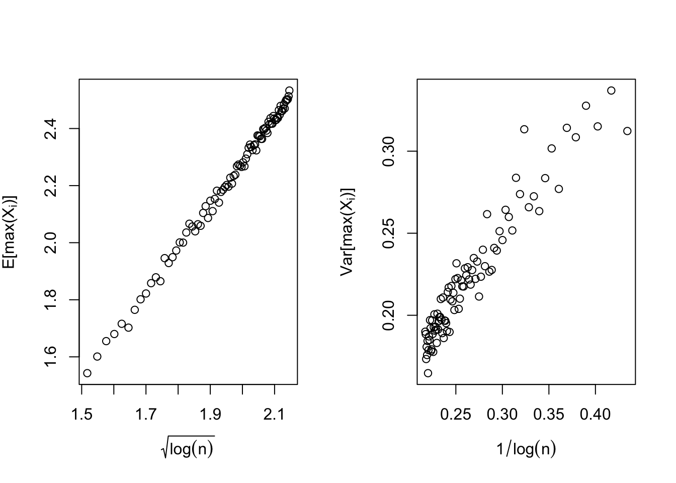
Consider $X \in R^{n}$ to be a Gaussian vector with covariance matrix $Σ$ . It is a well established result that the mean of $X^{(n)} = max_{i} X_{i}$ behaves roughly as $\sqrt{2 σ^{2} \log (n)}$ and the variance is bounded by $σ^{2} = max_{i \leq n} V a r (X_{i})$ . In order to obtain the former one can simply use Jensen’s inequality and optimize over $λ$ afterwards: $\frac{1}{λ} E [\log (e^{λ X^{(n)}})] \leq \frac{1}{λ} \log (E [e^{λ X^{(n)}}]) \leq \frac{1}{λ} \log (E [\sum_{i = 1}^{n} e^{λ X_{i}}]) \leq \frac{1}{λ} \log (n e^{\frac{λ^{2} σ^{2}}{2}})$ However, the variance bound requires extra work and can be proved via Poincaré’s Inequality mentioned earlier. Note that $f (Y) = max_{i} X_{i}$ where $Y = Σ^{- \frac{1}{2}} X$ is almost surely differentiable. Therefore, if we define $i^{*} = \arg max_{i} X_{i}$ then one can prove $f$ is $σ$ -Lipschitz via the chain rule and obtain the bound: $V a r (f) \leq E [| | \nabla f (Y) | |^{2}] = E [| | \frac{\partial X}{\partial Y} \frac{\partial f}{\partial X} | |^{2}] = E [| | Σ^{\frac{1}{2}} e_{i^{*}} | |^{2}] = E [e_{i^{*}}^{T} Σ e_{i^{*}}] \leq max_{i} Σ_{i, i} = σ^{2}$

Even though the concentration theorem suggest that $X^{(n)}$ is $σ$ -subgaussian however it’s sharpness is merely contingent upon Poincare’s inequality being unbeatable. In fact Talagrand⁸ proved an extention of Poincare’s inequality which provides a sufficient condition on how to beat it. In particular, the case of maximum over independent gaussians satisfy this condition thus concludes the following bound: $V a r (X^{(n)}) ≍ \frac{1}{\log (n)}$ Below is a simple simulation study with 1000 replications for each $n$ (between 10 to 100) which verifies the theoretical results.

Variance Bound for Spectral Norm

Thus far we proved $| | A | |_{o p}$ is 1-subgaussian, moreover its variance is bounded by one in the case of standard normal entries due to the fact that it’s 1-Lipschitz. However the following simulation indicates that spectral norm enjoys superconcentration and its variance behaves roughly as $(\sqrt{n} + \sqrt{m}) (1 / \sqrt{n} + 1 / \sqrt{m})^{\frac{1}{3}}$ , thus Lipschitz concentration once again has failed to capture the underlying truth!⁹ In this simulation $m = n$ and the variance was estimated over 1000 replications. Note that the slope of the line should be close to $- \frac{1}{3}$ .

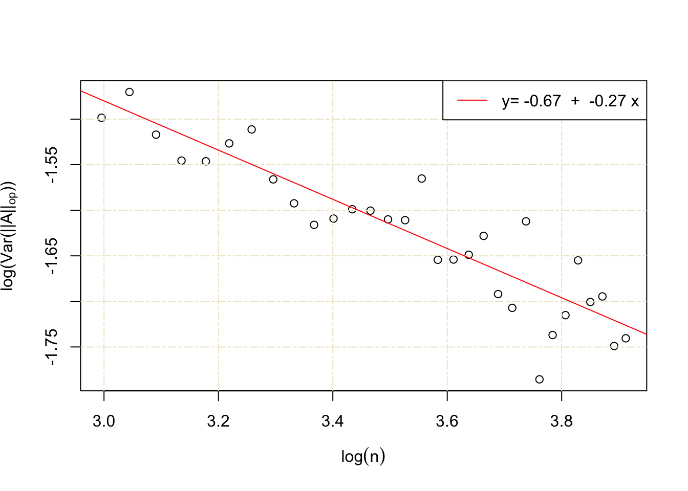It demands much more theory to prove this variance bound which I personally believe is one of the cases that the amount of effort that should be invested into proving it does not pay off proportionally!

One can look at High Dimensional Probability by Vershynin For a more comprehensive definition↩
This suprema can be written over a countable collection indexed by a set of dense vectors on $S^{n - 1}$ and $S^{m - 1}$ for those who are concerned about measurablity of spectral norm.↩
One might be suspicious about how maximum magically showed up and to the extent of which class of functions this theorem might hold. It’s in fact a well established result that superadditive functions (functions which $\frac{\partial^{2}}{\partial_{i} \partial_{j}} f \geq 0$ holds for all $i, j$ ) satisfy this inequality and maximum is just a special case.↩
The first tree methods can be found in Pollard. The latter can be found in Sec. 4 of High Dimesnional Probability lecture notes by Ramon Van Handel.↩
By running a simple approximation argument one may assume $f$ is sufficiently smooth and then extend the results to the general Lipschitz case.↩
The space of $R^{n \times m}$ can be equipped with either Frobenius or spectral norm distances in order for this to make sense.↩
There is a wonderful book by Chatterjee on this topic.↩
For a detailed derivation look at HDP by Ramon Van Handel Sec. 8.3↩
A proof of this can be found in chapter 9 of the book by Chatterjee mentioned earlier.↩